概述

逻辑回归和 softmax 回归都是用于分类问题的统计方法，属于广义线性模型的一部分。它们在本质上都是线性分类器，但应用于不同类型的分类问题。

逻辑回归

逻辑回归主要用于二分类问题。给定输入特征向量 $\mathbf{x}$，逻辑回归模型通过以下方式估计输入属于某一类别的概率：

1. 模型假设：使用线性组合 $z = \mathbf{w}^T \mathbf{x} + b$，其中 $\mathbf{w}$ 是权重向量，$b$ 是偏置。
2. 激活函数：应用逻辑函数（sigmoid 函数）$\sigma(z) = \frac{1}{1 + e^{-z}}$。
3. 输出：模型输出的概率 $P(y=1|\mathbf{x}) = \sigma(z)$。

逻辑回归通过最大化似然估计来估计模型参数。

Softmax 回归

Softmax 回归，也称为多项逻辑回归，是逻辑回归的扩展，用于多分类问题（即类别数大于 2）。其处理方式如下：

1. 模型假设：对于每一个类别 $k$，计算 $z_k = \mathbf{w}_k^T \mathbf{x} + b_k$。
2. 激活函数：应用 softmax 函数，将输入转换为概率分布：

   $$P(y=k|\mathbf{x}) = \frac{e^{z_k}}{\sum_{j} e^{z_j}}$$

3. 输出：通过 softmax 函数输出每个类别的概率。

与神经网络的关系

逻辑回归和 softmax 回归可以视为简单的神经网络：

• 逻辑回归相当于一个单一的神经元，使用 sigmoid 激活函数进行二分类。
• Softmax 回归相当于一个具有 softmax 激活函数的输出层，用于多分类。

在神经网络中，逻辑回归和 softmax 回归通常作为输出层使用：

• 逻辑回归常用作二分类神经网络的最后一层。
• Softmax 回归作为多分类神经网络的最后一层。

神经网络通过堆叠多个非线性层，可以学习复杂的特征表示，这使得它们比逻辑回归和 softmax 回归具有更强的表达能力和适应性。

应用与局限

• 应用：逻辑回归广泛用于医疗诊断、金融欺诈检测等二分类问题，其简单性和可解释性使其在很多实际应用中非常受欢迎。Softmax 回归常用于图像分类、文本分类等多分类问题，适用于类别数较多且相互排斥的场景。

• 局限：逻辑回归和 softmax 回归假设数据是线性可分的，因此在处理高度非线性的数据时表现不佳。它们对输入特征的质量十分敏感，需要良好的特征工程来提高性能，且难以捕捉复杂的特征之间的非线性关系，而神经网络可以通过多层结构克服这一局限。

在实践中，选择使用逻辑回归、softmax 回归还是更复杂的神经网络模型，通常取决于数据的具体特性、任务的复杂性以及计算资源的限制。

实践

介绍如何使用 PyTorch 构建一个简单的逻辑回归模型，以检测信用卡交易中的欺诈行为。此流程涵盖了数据加载、预处理、模型训练和评估等步骤。

数据集

使用 Kaggle 数据集 Credit Card Fraud Detection Dataset 2023，该数据集包含 2023 年欧洲持卡人的信用卡交易。该数据集包含超过 55 万条记录，为保护持卡人身份，数据已进行匿名化处理。该数据集的主要目的是促进欺诈检测算法和模型的开发，以识别潜在的欺诈交易。

导入库

导入所需的库，包括用于深度学习的 PyTorch，数据处理的 Pandas，数据可视化的 Seaborn 和 Matplotlib，以及用于数据预处理和评估的 Scikit-learn。

import os
import torch
from torch.utils.data import DataLoader, TensorDataset
import pandas as pd
import seaborn as sns
import matplotlib.pyplot as plt
from sklearn.model_selection import train_test_split
from sklearn.preprocessing import StandardScaler
from sklearn.metrics import confusion_matrix, precision_score, recall_score, f1_score

检查 CUDA 的可用性，以利用 GPU 加速计算：

if torch.cuda.is_available():
    print("CUDA is available! You can use GPU.")
    print("Current GPU:", torch.cuda.get_device_name(0))
else:
    print("CUDA is not available. You are using CPU.")

加载数据

使用 Pandas 加载数据集，并显示前五行数据：

df = pd.read_csv('../kaggle/input/creditcard_2023.csv')
df.head(5)

	id	V1	V2	V3	V4	V5	V6	V7	V8	V9	...	V21	V22	V23	V24	V25	V26	V27	V28	Amount	Class
0	0	-0.260648	-0.469648	2.496266	-0.083724	0.129681	0.732898	0.519014	-0.130006	0.727159	...	-0.110552	0.217606	-0.134794	0.165959	0.126280	-0.434824	-0.081230	-0.151045	17982.10	0
1	1	0.985100	-0.356045	0.558056	-0.429654	0.277140	0.428605	0.406466	-0.133118	0.347452	...	-0.194936	-0.605761	0.079469	-0.577395	0.190090	0.296503	-0.248052	-0.064512	6531.37	0
2	2	-0.260272	-0.949385	1.728538	-0.457986	0.074062	1.419481	0.743511	-0.095576	-0.261297	...	-0.005020	0.702906	0.945045	-1.154666	-0.605564	-0.312895	-0.300258	-0.244718	2513.54	0
3	3	-0.152152	-0.508959	1.746840	-1.090178	0.249486	1.143312	0.518269	-0.065130	-0.205698	...	-0.146927	-0.038212	-0.214048	-1.893131	1.003963	-0.515950	-0.165316	0.048424	5384.44	0
4	4	-0.206820	-0.165280	1.527053	-0.448293	0.106125	0.530549	0.658849	-0.212660	1.049921	...	-0.106984	0.729727	-0.161666	0.312561	-0.414116	1.071126	0.023712	0.419117	14278.97	0

检查数据集的信息，确保其完整性：

df.info()

输出

<class 'pandas.core.frame.DataFrame'>
RangeIndex: 568630 entries, 0 to 568629
Data columns (total 31 columns):
  #   Column  Non-Null Count   Dtype
---  ------  --------------   -----
  0   id      568630 non-null  int64
  1   V1      568630 non-null  float64
  2   V2      568630 non-null  float64
  3   V3      568630 non-null  float64
  4   V4      568630 non-null  float64
  5   V5      568630 non-null  float64
  6   V6      568630 non-null  float64
  7   V7      568630 non-null  float64
  8   V8      568630 non-null  float64
  9   V9      568630 non-null  float64
  10  V10     568630 non-null  float64
  11  V11     568630 non-null  float64
  12  V12     568630 non-null  float64
  13  V13     568630 non-null  float64
  14  V14     568630 non-null  float64
  15  V15     568630 non-null  float64
  16  V16     568630 non-null  float64
  17  V17     568630 non-null  float64
  18  V18     568630 non-null  float64
  19  V19     568630 non-null  float64
  20  V20     568630 non-null  float64
  21  V21     568630 non-null  float64
  22  V22     568630 non-null  float64
  23  V23     568630 non-null  float64
  24  V24     568630 non-null  float64
  25  V25     568630 non-null  float64
  26  V26     568630 non-null  float64
  27  V27     568630 non-null  float64
  28  V28     568630 non-null  float64
  29  Amount  568630 non-null  float64
  30  Class   568630 non-null  int64
dtypes: float64(29), int64(2)
memory usage: 134.5 MB

查看目标变量 Class 的分布情况：

df["Class"].value_counts()

输出

Class
0    284315
1    284315
Name: count, dtype: int64

数据预处理

去除不需要的列并对数据进行标准化处理：

X = df.drop(['id','Class'], axis=1)
y = df.Class

sc = StandardScaler()
X_scaled = sc.fit_transform(X)

将数据集划分为训练集和测试集：

X_train, X_test, y_train, y_test = train_test_split(X_scaled, y, test_size=0.2, random_state=42)

构建和训练模型

定义逻辑回归模型并进行训练：

class LogisticRegression(torch.nn.Module):
    def __init__(self, input_dim):
        super(LogisticRegression, self).__init__()
        self.linear = torch.nn.Linear(input_dim, 1)

    def forward(self, x):
        return torch.sigmoid(self.linear(x))

# 初始化模型
input_dim = X_train.shape[1]
model = LogisticRegression(input_dim)

# 定义损失函数和优化器
criterion = torch.nn.BCELoss()
optimizer = torch.optim.SGD(model.parameters(), lr=0.001)

训练模型并输出每 10 个 epoch 的损失：

num_epochs = 100
for epoch in range(num_epochs):
    for X_batch, y_batch in DataLoader(TensorDataset(torch.tensor(X_train, dtype=torch.float32), torch.tensor(y_train.values, dtype=torch.float32).unsqueeze(1)), batch_size=64, shuffle=True):
        outputs = model(X_batch)
        loss = criterion(outputs, y_batch)

        optimizer.zero_grad()
        loss.backward()
        optimizer.step()

    if (epoch+1) % 10 == 0:
        print(f'Epoch [{epoch+1}/{num_epochs}], Loss: {loss.item():.4f}')

输出

Epoch [10/100], Loss: 0.2015
Epoch [20/100], Loss: 0.1505
Epoch [30/100], Loss: 0.0612
Epoch [40/100], Loss: 0.1677
Epoch [50/100], Loss: 0.0866
Epoch [60/100], Loss: 0.0550
Epoch [70/100], Loss: 0.0663
Epoch [80/100], Loss: 0.0984
Epoch [90/100], Loss: 0.0452
Epoch [100/100], Loss: 0.0997

模型评估

在测试集上进行评估，计算准确率、精确率、召回率和 F1 分数，并绘制混淆矩阵和 ROC 曲线：

# 在测试集上进行评估
with torch.no_grad():
    y_pred = model(X_test_tensor)
    y_pred_labels = (y_pred > 0.5).float()

accuracy = (y_pred_labels.eq(y_test_tensor).sum() / y_test_tensor.shape[0]).item()
precision = precision_score(y_test_tensor, y_pred_labels)
recall = recall_score(y_test_tensor, y_pred_labels)
f1 = f1_score(y_test_tensor, y_pred_labels)

print(f'Accuracy: {accuracy * 100:.2f}%')
print(f'Precision: {precision:.2f}')
print(f'Recall: {recall:.2f}')
print(f'F1 Score: {f1:.2f}')

输出

Accuracy: 96.17%
Precision: 0.98
Recall: 0.94
F1 Score: 0.96

# 绘制混淆矩阵
cm = confusion_matrix(y_test_tensor, y_pred_labels)
plt.figure(figsize=(8, 6))
sns.heatmap(cm, annot=True, fmt="d", cmap="Blues",
            xticklabels=["Predicted No Fraud", "Predicted Fraud"],
            yticklabels=["Actual No Fraud", "Actual Fraud"])
plt.ylabel('Actual')
plt.xlabel('Predicted')
plt.title('Confusion Matrix')
plt.show()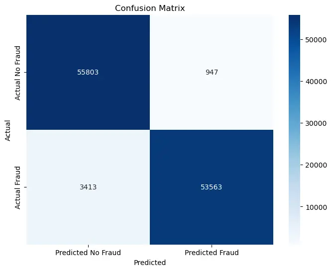

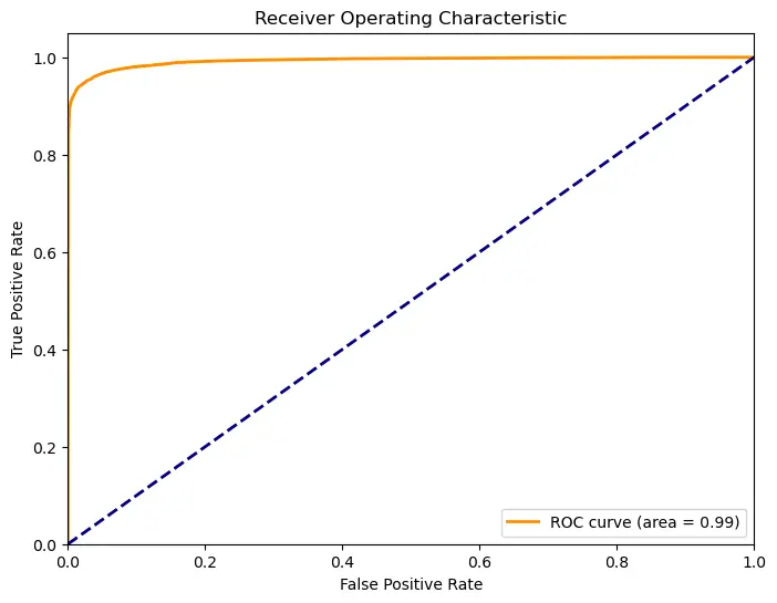
# 计算ROC曲线和AUC值
fpr, tpr, thresholds = roc_curve(y_test_tensor, y_pred)
roc_auc = auc(fpr, tpr)

# 绘制ROC曲线
plt.figure(figsize=(8, 6))
plt.plot(fpr, tpr, color='darkorange', lw=2, label='ROC curve (area = %0.2f)' % roc_auc)
plt.plot([0, 1], [0, 1], color='navy', lw=2, linestyle='--')
plt.xlim([0.0, 1.0])
plt.ylim([0.0, 1.05])
plt.xlabel('False Positive Rate')
plt.ylabel('True Positive Rate')
plt.title('Receiver Operating Characteristic')
plt.legend(loc="lower right")
plt.show()

贡献者

• fanwendi8

版权所有

版权归属：fanwendi8

本文链接：/machine-learning/81hq20pl/

许可证：署名-非商业性-禁止演绎 4.0 国际 (CC-BY-NC-ND-4.0)