概述

决策树是一种常用的监督学习算法，适用于分类和回归任务。它通过一系列的决策规则将数据集划分成更小的子集，从而形成一个树状结构。决策树模型具有高度的解释性，能够直观地展示决策过程。

决策树的基本形式

• 节点类型：

  • 决策节点：表示对某个特征的测试。
  • 叶节点：代表分类结果或回归输出。

• 生成过程：

  • 选择最佳特征进行数据划分，常用的准则包括信息增益、信息增益率和基尼指数。
  • 递归地在每个子集上进行上述过程，直至满足停止条件（例如，节点纯度达到阈值或树深度限制）。

决策树的特性

• 简单直观：易于理解和解释，特别适合展示复杂决策逻辑。
• 灵活性：能够处理数值型和类别型数据，并且不要求特征间的线性关系。

决策树的优缺点

• 优点：

  • 解释性强：可以清晰地展示决策路径。
  • 无需数据预处理：不需要特征缩放或归一化。
  • 能够处理多种数据类型：包括数值和类别数据。

• 缺点：

  • 易过拟合：特别是在树的深度不加限制时。
  • 不稳定性：小的扰动可能导致树结构的显著变化。
  • 偏差-方差权衡：单一决策树可能不足以捕获数据的复杂模式，通常结合集成方法（如随机森林）来提升性能。

与其他模型的比较

• 与线性模型相比：决策树无需假设数据的线性关系，更适合非线性和复杂的决策边界。
• 与神经网络相比：决策树模型更易于解释，但对复杂模式的捕捉能力相对较弱。

应用与扩展

• 应用场景：广泛用于金融风险评估、医疗诊断、市场营销等领域。
• 扩展方法：通过集成技术（如随机森林、梯度提升树）提高模型的泛化能力和稳定性。

总之，决策树是一种强大的模型，提供了良好的可解释性和灵活性。在现代机器学习中，决策树的变体和集成方法进一步增强了其应用广度和深度。

实践

介绍如何使用 Scikit-learn 构建一个简单的决策树模型，以检测信用卡交易中的欺诈行为。此流程涵盖了数据加载、预处理、模型训练和评估等步骤。

数据集

使用 Kaggle 数据集 Credit Card Fraud Detection Dataset 2023，该数据集包含 2023 年欧洲持卡人的信用卡交易。该数据集包含超过 55 万条记录，为保护持卡人身份，数据已进行匿名化处理。该数据集的主要目的是促进欺诈检测算法和模型的开发，以识别潜在的欺诈交易。

导入库

导入所需的库，包括用于数据处理的 Pandas，数据可视化的 Seaborn 和 Matplotlib，以及用于模型训练和评估的 Scikit-learn。

import pandas as pd
import seaborn as sns
import matplotlib.pyplot as plt
from sklearn.model_selection import train_test_split
from sklearn.metrics import confusion_matrix, roc_curve, auc, classification_report
from sklearn.tree import DecisionTreeClassifier as DTC, plot_tree

加载数据

使用 Pandas 加载数据集，并显示前五行数据：

df = pd.read_csv('../kaggle/input/creditcard_2023.csv')
df.head(5)

	id	V1	V2	V3	V4	V5	V6	V7	V8	V9	...	V21	V22	V23	V24	V25	V26	V27	V28	Amount	Class
0	0	-0.260648	-0.469648	2.496266	-0.083724	0.129681	0.732898	0.519014	-0.130006	0.727159	...	-0.110552	0.217606	-0.134794	0.165959	0.126280	-0.434824	-0.081230	-0.151045	17982.10	0
1	1	0.985100	-0.356045	0.558056	-0.429654	0.277140	0.428605	0.406466	-0.133118	0.347452	...	-0.194936	-0.605761	0.079469	-0.577395	0.190090	0.296503	-0.248052	-0.064512	6531.37	0
2	2	-0.260272	-0.949385	1.728538	-0.457986	0.074062	1.419481	0.743511	-0.095576	-0.261297	...	-0.005020	0.702906	0.945045	-1.154666	-0.605564	-0.312895	-0.300258	-0.244718	2513.54	0
3	3	-0.152152	-0.508959	1.746840	-1.090178	0.249486	1.143312	0.518269	-0.065130	-0.205698	...	-0.146927	-0.038212	-0.214048	-1.893131	1.003963	-0.515950	-0.165316	0.048424	5384.44	0
4	4	-0.206820	-0.165280	1.527053	-0.448293	0.106125	0.530549	0.658849	-0.212660	1.049921	...	-0.106984	0.729727	-0.161666	0.312561	-0.414116	1.071126	0.023712	0.419117	14278.97	0

确保数据集的完整性：

df.info()

输出

<class 'pandas.core.frame.DataFrame'>
RangeIndex: 568630 entries, 0 to 568629
Data columns (total 31 columns):
  #   Column  Non-Null Count   Dtype
---  ------  --------------   -----
  0   id      568630 non-null  int64
  1   V1      568630 non-null  float64
  2   V2      568630 non-null  float64
  3   V3      568630 non-null  float64
  4   V4      568630 non-null  float64
  5   V5      568630 non-null  float64
  6   V6      568630 non-null  float64
  7   V7      568630 non-null  float64
  8   V8      568630 non-null  float64
  9   V9      568630 non-null  float64
  10  V10     568630 non-null  float64
  11  V11     568630 non-null  float64
  12  V12     568630 non-null  float64
  13  V13     568630 non-null  float64
  14  V14     568630 non-null  float64
  15  V15     568630 non-null  float64
  16  V16     568630 non-null  float64
  17  V17     568630 non-null  float64
  18  V18     568630 non-null  float64
  19  V19     568630 non-null  float64
  20  V20     568630 non-null  float64
  21  V21     568630 non-null  float64
  22  V22     568630 non-null  float64
  23  V23     568630 non-null  float64
  24  V24     568630 non-null  float64
  25  V25     568630 non-null  float64
  26  V26     568630 non-null  float64
  27  V27     568630 non-null  float64
  28  V28     568630 non-null  float64
  29  Amount  568630 non-null  float64
  30  Class   568630 non-null  int64
dtypes: float64(29), int64(2)
memory usage: 134.5 MB

查看目标变量 Class 的分布情况

df["Class"].value_counts()

输出

Class
0    284315
1    284315
Name: count, dtype: int64

数据预处理

去除不需要的列，然后将数据集划分为训练集和测试集。值得注意的是，决策树模型不要求输入数据进行标准化或归一化，因为它基于树结构，不受特征尺度的影响。

X = df.drop(['id', 'Class'], axis=1)
y = df.Class

X_train, X_test, y_train, y_test = train_test_split(X, y, test_size=0.2, random_state=42)

构建和训练模型

定义并训练决策树模型：

dtc = DTC(random_state=42)
dtc.fit(X_train, y_train)

可视化决策树

plt.figure(figsize=(20, 5))
plot_tree(dtc, filled=True, feature_names=X.columns, class_names=["No Fraud", "Fraud"], rounded=True, fontsize=8, max_depth=3)
plt.title("Decision Tree")
plt.show()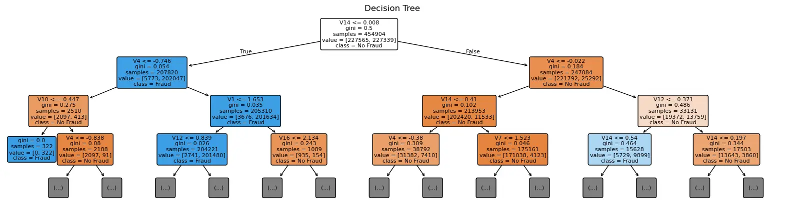

模型评估

进行预测并使用 classification_report 输出评估指标：

y_pred = dtc.predict(X_test)

print(classification_report(y_test, y_pred, target_names=["No Fraud", "Fraud"], digits=4))

	precision	recall	f1-score	support
No Fraud	0.9990	0.9972	0.9981	56750
Fraud	0.9972	0.9990	0.9981	56976
accuracy			0.9981	113726
macro avg	0.9981	0.9981	0.9981	113726
weighted avg	0.9981	0.9981	0.9981	113726

绘制混淆矩阵

cm = confusion_matrix(y_test, y_pred)
plt.figure(figsize=(8, 6))
sns.heatmap(cm, annot=True, fmt="d", cmap="Blues",
            xticklabels=["Predicted No Fraud", "Predicted Fraud"],
            yticklabels=["Actual No Fraud", "Actual Fraud"])
plt.ylabel('Actual')
plt.xlabel('Predicted')
plt.title('Confusion Matrix')
plt.show()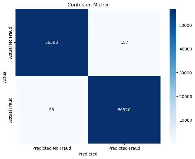

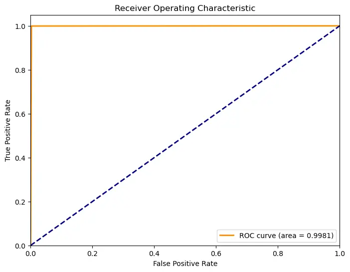
计算并绘制 ROC 曲线和 AUC 值：

fpr, tpr, thresholds = roc_curve(y_test, y_pred)
roc_auc = auc(fpr, tpr)

plt.figure(figsize=(8, 6))
plt.plot(fpr, tpr, color='darkorange', lw=2, label='ROC curve (area = %0.4f)' % roc_auc)
plt.plot([0, 1], [0, 1], color='navy', lw=2, linestyle='--')
plt.xlim([0.0, 1.0])
plt.ylim([0.0, 1.05])
plt.xlabel('False Positive Rate')
plt.ylabel('True Positive Rate')
plt.title('Receiver Operating Characteristic')
plt.legend(loc="lower right")
plt.show()

贡献者

• fanwendi8

版权所有

版权归属：fanwendi8

本文链接：/machine-learning/aqmg132k/

许可证：署名-非商业性-禁止演绎 4.0 国际 (CC-BY-NC-ND-4.0)